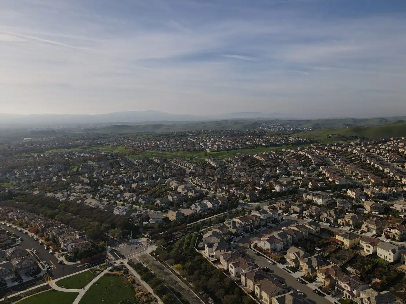
If you're scoping a curb-appeal or parcel-condition feature for an AVM, the first question your imagery vendor will ask is what ground sample distance you're working with. That number sets the hard ceiling on what your model can ever resolve in a single pixel. Get it wrong and the feature doesn't carry usable signal, no matter how good the rest of the pipeline is.
What GSD actually controls
Ground sample distance is the size of the area one pixel covers on the ground. At 1 m GSD, each pixel is a 1 m by 1 m patch. That's fine for confirming a building footprint or counting rooftops in a block, but it's not fine for anything you'd call curb appeal. A driveway crack, a tarped roof section, an overgrown yard versus a maintained one: these are features that span a handful of pixels at best once you're above 1 m. Below that, they start blurring into the parcel around them, and your embedding model ends up learning noise instead of condition.
Sub-meter imagery changes what's resolvable. At 0.5 m GSD, a single-family lot that might be 20 m by 40 m resolves into roughly 1,600 pixels, enough for a model to pick up on surface texture differences between a kept lawn and bare dirt, distinguish a paved driveway from gravel, or flag a pool, a detached structure, or storage clutter that never made it onto the tax roll. That's the resolution tier where parcel-level signal starts to look like signal and not like a smudge.
Why "good enough for a map" isn't good enough for a model
A lot of free and low-cost imagery sits in the 0.6 m to 3 m range, which is plenty for a basemap, a flood layer, or a land-use classification at the neighborhood scale. The trouble is that those use cases are forgiving of exactly the detail an AVM feature needs. A 3 m pixel can still tell you "there's a house here." It cannot tell you whether that house has a sagging carport out back or a freshly resurfaced driveway out front, and those are the kind of details that move comps in the field but never show up in a tabular record.
This is the gap most AVM teams run into once they decide tabular fields alone aren't capturing neighborhood and parcel context. You can engineer features from permits, assessor photos, or Street View crops, but none of those give you a consistent, wall-to-wall view refreshed on a schedule you control. Satellite and aerial imagery at 0.5 m or finer is the only input that covers every parcel in your book at the same cadence, which matters more for a production feature than it sounds like it should. A model trained on inconsistent coverage learns inconsistent things.
RGB is usually enough, cadence matters more than spectral bands
For curb-appeal and parcel-context scoring specifically, plain RGB at sub-meter GSD does most of the work. Curb-appeal scoring cares about upkeep, clutter, and surrounding lot condition: the kind of details an appraiser would clock walking the block, all visible in three color bands. Near-infrared and other spectral bands earn their keep in crop-health or moisture-detection work, where the signal lives outside what the eye can see. A yearly refresh is usually the right cadence too. Curb appeal doesn't swing week to week the way a construction site does, so there's no reason to pay for a revisit rate you don't need just because it's available.
If you're building this out as an embedding you feed into an existing valuation model rather than a standalone visual-inspection product, the imagery requirement is really just the floor: 0.5 m or better, annual, RGB, keyed to your parcel IDs so it joins cleanly to the records you already have. AVM Imagery is built around that exact spec, delivering a vector per property rather than a raw image your pipeline has to process from scratch.
If your team is weighing whether to add this kind of signal to your next model iteration, it's worth a look.